Generation of Signals using MATLAB/Python

Dr. Hari V S
Department of Electronics and Communication
College of Engineering Karunagappally

What You will Learn

• You will learn about various energy signals and their generation using MATLAB and python.

Signal Generation using MATLAB

MATLAB arrays are used to generate finite energy signals. It should be understood that the signals so generated are discrete in time and amplitude.

Sinusoidal Signal

Consider the sinusoidal signal $x=sin(t)$, which is nothing but a single tone, with the help of the MATLAB code below.
t=linspace(0,10,5000);
x=sin(t);
plot(t,x);
grid;
The execution of the code will result in the signal, shown below.

Amplitude Modulated Signal

The above low frequency tone is used to modulate a sinusoidal carrier $y$ of ten times the original frequency. i.e. $y=sin(10t)$. The amplitude modulated signal $am(t)$ is obtained as \begin{equation} am(t)=x*y+y \end{equation}Such an AM signal is generated with the help of the MATLAB code, given below.
t=linspace(0,10,5000);
x=sin(t);
y=sin(10*t);
am=x.*y+y;
plot(t,am);
grid;
The resulting amplitude modulated signal is shown below.

Square Pulse using MATLAB

Square pulses are used in digital and radar communication, local area networks, analog signal processing etc., though their use is much limited by the wide frequency spectrum. Such a pulse of height one unit is realized by the MATLAB code, listed below.
T=5;
t1=linspace(-T,-0.5*T,2000);
t2=linspace(-0.5*T,0.5*T,2000);
t3=linspace(0.5*T,T,2000);
t=horzcat(t1,t2,t3);
x=horzcat(zeros(1,length(t1)),ones(1,length(t2)),zeros(1,length(t1)));
plot(t,x);
grid;
the above code will create a pulse that is centered about the origin with width $5$ units. The first line dictates that half of the time base is $5$ units. The code in the fifth lines concatenates $t_1$, $t_2$ and $t_3$ to form the time base $t$, using the $horzcat$ function. Vectors of zeros and ones are appropriately conacted in the xixth line to genertae the pulse $x$. The function is then plotted with grid on the GUI. The plot is shown below.

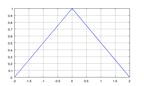
Triangular Signal using MATLAB

The triangular function \begin{equation}x(t)=1-\frac{|t|}{T}\end{equation} Let us look at the code that returns a triangular signal, centered about the origin.
T=2;
t=linspace(-1*T,T,5000);
triang=1-abs(t)/T;
plot(t,triang);
grid;
Observe the signal in the figure below.

Signal Generation using Python

The scipy arrays are used to generate many discrete signals, the same way MATLAB was used earlier. The following code shows the generation of a sinusoid.

from scipy import *
from pylab import *
t=linspace(0,10,1000)
x=sin(t)
plot(t,x)
grid('on')
savefig('sinusplot.pdf')
show()

The above code generates a sinusoid and saves as a .pdf files in the current working directory. The GUI looks like what is shown below.

Amplitude Modulated Signal using Python

The above low frequency tone is used to modulate a sinusoidal carrier $y$ of ten times the original frequency. i.e. $y=sin(10t)$. The amplitude modulated signal $am(t)$ is obtained with the following code
from scipy import *
from pylab import *
t=linspace(0,10,1000)
x=sin(t)
y=sin(10*t)
am=x*y+y
plot(t,am)
grid('on')
savefig('amplot.pdf')
show()
The plot of the AM signal generated is shown below.

Square Pulse using Python

The following code generates a pulse.
from scipy import *
from pylab import *
N1=100
N2=40
x=concatenate([zeros(N1),ones(N2),zeros(N1)])
plot(x)
grid('on')
savefig('pulsesig.pdf')
show()
The pulse signal is shown below.

Triangular Signal using Python

The following Python code generates the triangular signal.
from scipy import *
from pylab import *
T=2
t=linspace(-1*T,T,5000)
triang=1-abs(t)/T
plot(t,triang)
grid('on')
savefig('triang.pdf')
show()

What You Learned

• You learned the use of MATLAB and python arrays to simulate the energy signals.